3. Creating a simple model

In this exercise we will be creating a simple model with /docs/user_manual/processing/modeler. In this exercise you will work with Model Builder yourself. This is an important tool since you will use it often in Chapter 3 of this practical. Here you will automate a series of operations so that they can be executed with just one click. It will also allow you to make changes to parameter settings and then quickly re-run the model. This allows you to compare changes in your model output and link them to the changes that you made earlier. In this exercise, you will create a model that determines the Topographic Position Index (TPI) of a DEM. The TPI is given by the equation:

\[TPI=DEM-\mathrm{focalmean}\left(DEM,annulus,r_i,r_o\right)\]

The TPI can be used to determine whether a location is on a ridge or valley. This can be useful when you are creating your own adaptation strategies!

As you can see in Fig. 3.1, the TPI can differ, based on the radius. This is useful so you can distinguish between large and small features.

Fig. 3.1 Topographic index depends on Neighborhood size. (https://landscapearchaeology.org/2019/tpi/)

3.1. implementing the model with r.neighbors

Since is a bit difficult and has different versions, the preferred way to implement the TPI is to use r.neighbors. This is a focal statistics algorithm: it takes all cells in a neighborhood around a cell and uses them to calculate the value for a cell.

3.1.1. Follow Along: Adding the annulus mask script to the toolbox

The r.neighbors algorithm does not support an annulus as area by default. However, it provides the possibility to use a mask file. That is a .txt file that for \(r_i=1,r_o=3\) looks something like this:

0 0 0 1 0 0 0
0 1 1 1 1 1 0
0 1 1 1 1 1 0
1 1 1 0 1 1 1
0 1 1 1 1 1 0
0 1 1 1 1 1 0
0 0 0 1 0 0 0

Where all \(1\)’s are taken into account. The script that we need creates this file for us. In Follow Along: Creating a script for the mask file we will be making this script ourselves. You can also directly copy it from the convenience scripts.

1. extract the convenience scripts to a location of your choice.

2. In the processing toolbox, click the Add script to toolbox… and select the annulus_r_neighbors.py file.

   The script should now be added to your toolbox.

   

3.1.2. Follow Along: Getting the model inputs

1. In the Processing toolbox, select ► Create new Model

   

   The following window will show:

   

   Fig. 3.2 The canvas. Enter 01_update_landuse as name and pre-processing as group.

   Our TPI model needs three inputs:

   • A Digital Elevation Model (DEM) raster

   • The inner radius for the zonal statistics

   • The outer radius for the zonal statistics

2. In the Inputs pane, scroll down until you see Raster Layer. drag it into the model view. The following dialog will show:

   

   Enter DEM as name and press OK.

   Note

   The checkboxes define how the inputs are shown when you open a model:

   • Your created model will not run without Mandatory inputs

   • advanced inputs will be under a drop-down menu

3. Drag a Number into the modeler. Give it a:

   • Description: Outer radius

   • Number type: Integer

   • Minimum value: 1

   • Default value: 3

   Your modeler should now look like this:

   

   Fig. 3.3 Model with only inputs

   Tip

   Snapping You can enable snapping by View ► Enable snapping

4. |TY| Add another input for the inner radius.

5. Name the model Topographic Position Index (TPI) and Save it with a logical name such as tpi.model3

6. close the modeler for now

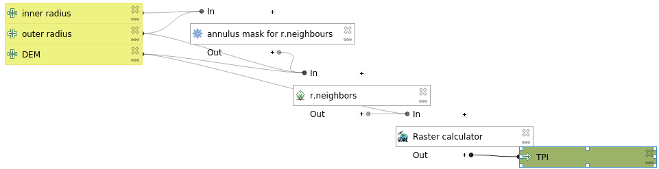
3.1.3. Adding the processes to the TPI model

Now we have all the processes we need, it is time to add them to our model!

1. Click Algorithms (highlighted in Fig. 3.3).

2. Search for your script and drag it into the modeler. Fill it in like this:

   

   You can change the type of variable by clicking the highlighted . You can then choose from:

   • Value A value

   • Input An input to your model ()

   • Algorithm output The output of an algorithm

   • Pre-calculated value An expression that will be evaluated when you run the model

3. Next, drag in the r.neighbors algorithm. The mask option we are using is an advanced parameter. Click the Show avancedparameters button. Then fill it in like this:

   • Using model input: DEM

   • Neighborhood operation [optional]: average

   • Neighborhood size (must be odd) [optional]: outer radius

   • File containing weights [optional]: "annular mask" from algorithm "annulus mask for r.neighbors"

   press OK

Note

For some reason, the native raster calculator does not work well with output of Saga or Grass algorithms. Please use the gdalrastercalculator for this exercise. Instructions are still added, because you may find it more intuitive to use than the GDAL version later on in the manual. However, I used the gdalrastercalculator for everything.

1. Drag the gdalrastercalculator into the view. Fill in the dialog as follows:

   • Input layer A: DEM

   • Number of raster band for A: 1 This is for multi-band rasters. Since our raster only has one band, we want that to be \(1\).

   • Input layer B: "neighbors" from algorithm "r.neighbors"

   • Number of raster band for B: 1

   • Calculation in gdalnumeric syntax: A-B

   • Calculated: TPI

   Your model should now look like this:

   

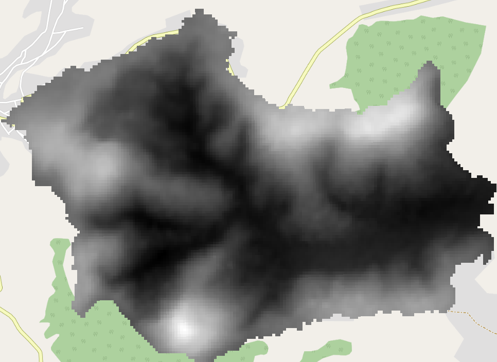
2. Run your model with \(r_i=62,r_o=67\). Your output should look like this:

3.2. Implementing the algorithm with Focal statistics

Warning

The following section was written for QGIS with SAGA 7.8. This version has different algorithms available than version 7.3. In that case, use the :r.neighbors algorithm.

1. In the Processing toolbox, select ► Create new Model

   

   The following window will show:

   

   Our TPI model needs three inputs:

   • A Digital Elevation Model (DEM) raster

   • The inner radius for the zonal statistics

   • The outer radius for the zonal statistics

2. In the Inputs pane, scroll down until you see Raster Layer. drag it into the model view. The following dialog will show:

   

   Enter DEM as name and press OK.

   Note

   The checkboxes define how the inputs are shown when you open a model:

   • Your created model will not run without Mandatory inputs

   • advanced inputs will be under a drop-down menu

3. Drag a Number into the modeler. Give it a:

   • Description: Outer radius

   • Number type: Integer

   • Munimum value: 1

   • Default value: 3

   Your modeler should now look like this:

   

   Fig. 3.4 Model with only inputs

   Tip

   Snapping You can enable snapping by View ► Enable snapping

4. Now, we are going to include our first algorithm.

   1. Click Algorithms (highlighted in Fig. 3.4).

   2. Search for Focal Statistics, drag it into the view and fill in the pop-up window as follows:

      • Under Grid, press the drop-down and select Model Input. It should be on DEM already since this is the only raster type model input.

      • Include Center Cell: No

      • Kernel Type: [1] Circle

      • Radius: Outer radius

      • the rest on default settings

   3. Press OK

      Your model should now look like this (with some rearranging):

      

Note

For some reason, the native raster calculator does not work well with output of Saga algorithms. Please use the gdalrastercalculator for this exercise. Instructions are still added, because you may find it more intuitive to use than the GDAL later on in the manual

1. Drag the gdalrastercalculator into the view. Fill in the dialog as follows:

   • Input layer A: DEM

   • Number of raster band for A: 1 This is for multi-band rasters. Since our raster only has one band, we want that.

   • Input layer B: "Mean value" from algorithm "Focal Statistics"

   • Number of raster band for B: 1

   • Calculation in gdalnumeric syntax: A-B

   • Calculated: TPI

Raster calculator

1. Drag the Raster calculator into the view. Fill in the dialog as follows:

   • Expression: "DEM@1"-"'Mean Value' from algorithm 'Focal Statistics'@1". Get the names by double-clicking them in the Layers list.

   • Reference Layers (…): … ►`|checkbox|:guilabel:`DEM.

   • Output: TPI

   and press OK.

   Note

   In DEM@1, the @1 refers to Band 1. Thus, the raster calculator supports operations on rasters with multiple bands.

1. Press OK to add it to the model. It should now look like this:

   

2. Before we can save our model, we have to give it a name. Below Model Properties, give it the Name Topographic Position Index (TPI)

3. Save your model by pressing the icon or Ctrl+S. Give it a descriptive name.

3.3. Running the model

Note

Currently (Oct 2021), layers from a GeoPackage cannot be selected as raster inputs in the Graphical Modeler. See the related Feature request and a Possible workaround . However, we will be working around this by loading our data into the project first.

1. Load the Hadocha_dem layer into your map if it isn’t there yet.

2. Now we have created the model, it is time to run it! There are two ways to do so:

   1. From within the Graphical Modeler:

      Press the button or F5.

   2. From the Processing Toolbox:

      Notice that there is a new drop-down menu labeled Models. There, your model named Topographic Position Index is shown. Run it like any other tool!

3. Either way, now select Hadocha_DEM as DEM. and outer radius 3. Run the model and your output should look like this:

   

3.4. In Conclusion Wrapping up

Now, you have learned how to use the graphical modeler and to calculate the Topographic Position Index. Both are very useful. We will excessively use the Graphical Modeler later for the MMF erosion model, and you could use the TPI for determining where to apply specific measures.