4.2. Pre-processing the data

In GIS you always need to process the raw data, to make it suitable as input for your application. We consider this as the first step in the process. In total there are three different phases: the pre-processing phase, where the input data will be created from the raw data. The second phase is the processing, where every step in the MMF method will be completed. The last phase is combining the different steps to the complete model.

Fig. 4.1 Flowchart for the complete preprocessing workflow.

4.2.1. Managing files for processing

Even though GeoPackages are very useful for easy sharing of data, there are some small quirks when opening rasters from them for models we made ourselves. Therefore, we will be dumping all our rasters in a folder.

1. Create a folder 01_input inside GIS_files.

4.2.2. Follow Along: Updating Hadocha_landuse

Since updating the landuse map has the shortest workflow, we’ll work on that first. The data in data/Hadocha_landuse.xlsx still needs some editing.

4.2.2.1. Pre-processing the tabular data

1. Open data/Hadocha_data.xlsx in a spreadsheet editor like Libreoffice Calc

2. In the landuse_properties_table tab, have a look at the data. As you can see, the Cropland data is not annual, but hs different values for each month. Since the MMF model is annual, we need annual data. Calculate the annual intercepted rainfall (\(A\)) by:

   (4.1)\[A = \frac{A_{sow}*M_{sow}+A_{grow}*M_{grow}+A_{after}*M_{after}}{12}\]

   Where \(A_{sow,grow,after}\) is the intercepted rainfall for that period (sowing, growing and after harvest) and \(M_{sow,grow,after}\) the number of months in each period.

3. Calculate the other other factors by substituting \(A\) in (4.1)

4. Make sure to name the row Cropland

Note

The rows will later be used to perform a qgisjoinattributestable operation. This will give the Cropland features of Hadocha_landuse the values of landuse_properties_table. This will only work if both rows have exactly the same names.

4.2.2.2. Joining the data

Even though the join operation is only a single operation, we will put it inside a model, so we can immediately rasterize the data afterwards.

1. Create a new model named 01 update landuse and Save it.

2. We need the following inputs:

   1. Vector Layer

      • Description landuse

      • Geometry type Polygon

      • Mandatory

      • Advanced

   2. Vector field

      • Description Landuse join field

      • Parent layer Landuse

      • Allowed data type String

      • Accept multiple fields

      • Default value: FEATURE

   3. Vector Layer

      • Description Landuse properties

      • Geometry type No geometry required

   4. Vector field

      • Description landuse properties join field

      • Parent layer Landuse properties

      • Allowed data type String

      • Accept multiple fields

      • Default value: Landuse

3. Drag the qgisjoinattributestable algorithm into the modeler.

   • Input layer: Landuse

   • Table field: Landuse join field

   • Input layer 2: Landuse properties

   • Table field 2: Properties table join field

   • Joined layer [optional]: Landuse_joined

4. Run the model and look at the attribute table. It should look like this: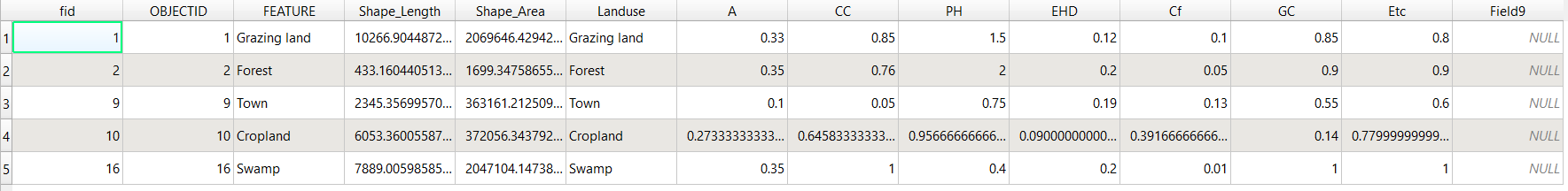

   

   Note that there may be additional, unnecessary columns like Field9 with all NULL values. These are okay.

   Note

   It may be that your Cropland row will have all NULL values. If that is the case, check:

   1. If you have calculated the values

   2. It may be that the values don’t load if they are a formula. This should be a bug and is hopefully solved soon. Replace your formulas with the resulting numbers!

4.2.2.3. Rasterizing the results

Now, we will be going to rasterize all our outputs. This is normally done by the gdalrasterize process. To make this easier, two convenience scripts have been added: one that allows you to rasterize a single vector layer with the same extent and pixel size as another raster layer, and one that allows you to do the same for multiple rasters. We will be using the batch rasterizing script, and you can use the other one later if you need to.

1. Add the batch_rasterize_final.py convenience script to the toolbox. like you did in Follow Along: Adding the annulus mask script to the toolbox.

2. We will need another input Raster Layer reference layer. This is the layer that will be used to calculate the extent. Open up 01_update_landuse again and add it.

3. Also add another Vector field input with:

   • Description Rasterize fields

   • Parent layer landuse properties table

   • Allowed data type number

   • Accept multiple fields

   • Select all fields by default

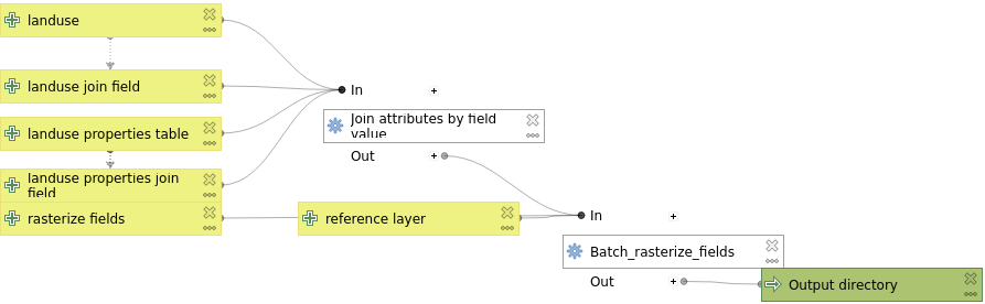
4. drag in the Batch_rasterize_fields script you added and set:

   • like raster reference layer

   • vector "Joined layer" from algorithm "Join attributes by field value"

   • fields to select rasterize fields

   • Output directory Output directory

   Your model should now look like this:

   

5. We also want our output to be automatically saved to a non-temporary location. Double click the Output directory output and set it to a location:

   

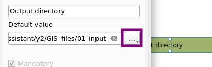
   Fig. 4.2 Setting a default output for intercepted rainfall. 01_input is a folder, not a GeoPackage.

6. Run the model and verify that the output has data values for all areas.

4.2.3. Follow Along: Updating Hadocha_soil

Now it is time to start working on our soil layer! Because there is a swamp (landuse) which has quite different properties than the surrounding land, we will first put that in our map

4.2.3.1. Follow Along: Adding Swamp to the Soil map

1. Create a new model. Name it 02 Update Soil

2. Give it the following inputs:

   1. Vector Layer: Soil

   2. Vector Layer: Landuse

3. Now, we want to select the Swamp feature from Landuse. Drag the Extract by Attribute process into the modeler.

   • Input layer: Landuse

   • Selection attribute: FEATURE

   • Operator: =

   • Value [optional]: Swamp

   Also give Extracted (attribute) a name and Run the model. Your resulting layer should only be the swamp.

   Note

   It is good practice to run and check your model after each step/algorithm you put in. This will not really be said from now on, but we expect you to do this. Also if your final output is wrong, go back in the model and check every earlier output for an error.

4. Next, we want to combine our Swamp into the Soil layer. Drag a qgisunion into the modeler with:

   • Input layer: Soil

   • Overlay layer: "Extracted (attribute)" from algorithm "Extract by attribute"

   Run the model and check the output attribute table.

   

   Notice that there is a field TEXTURE and a field FEATURE. In the next step, we will combine these, such that the TEXTURE for all features that have FEATURE=='Swamp' will be Swamp.

5. Drag in the qgisfieldcalculator tool into the model.

   • Input layer: "Union" from "Union"

   • Field name: TEXTURE

   • Result field type: String

   • Result field length: 16 This is the maximum length that the resulting field can have in characters

   • Formula: IF("FEATURE"='Swamp',"FEATURE","TEXTURE")

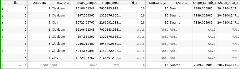
   Now, let’s break this down a bit: Double quotes ("") indicate a field. For example, "FEATURE" will take values of 'Swamp' or NULL. Single quotes ('') indicate a String. This is just a sequence of letters such as 'Swamp'. The IF() works like: IF(something is true, then this, otherwise this). The resulting attribute table should look like this:

   

   This still has some unnecessary fields, and multiple features that have the same TEXTURE.

6. Drag in the qgisaggregate operation. This is a sort of qgisdissolve operation, but it offers more control over the output. Fill it in like this:

   • Input layer: "Calculated from algorithm "Field calculator"

   • Group by expression: TEXTURE

   • Aggregates: Click the Add new field button to add a new field. and fill it in like this:

     Source expression	Aggregate Function	Name	Type	Length
     “TEXTURE”	first_value	TEXTURE	Text (string)	16

   Tip

   in stead of adding the above fields manually, you can also Load fields from a similar layer.

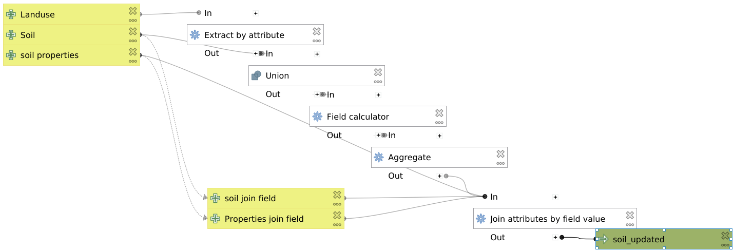
   Your resulting layer should have a single column named TEXTURE and look like this:

   

4.2.3.2. Try Yourself Join soil properties and rasterize

The only thing we need to do now, is to join the excel table and rasterize the results This is exactly the same as we did for the landuse maps, so we will give less instructions.

1. Change the model such that soil properties are joined to the map. For reference, see Joining the data.

   Hint

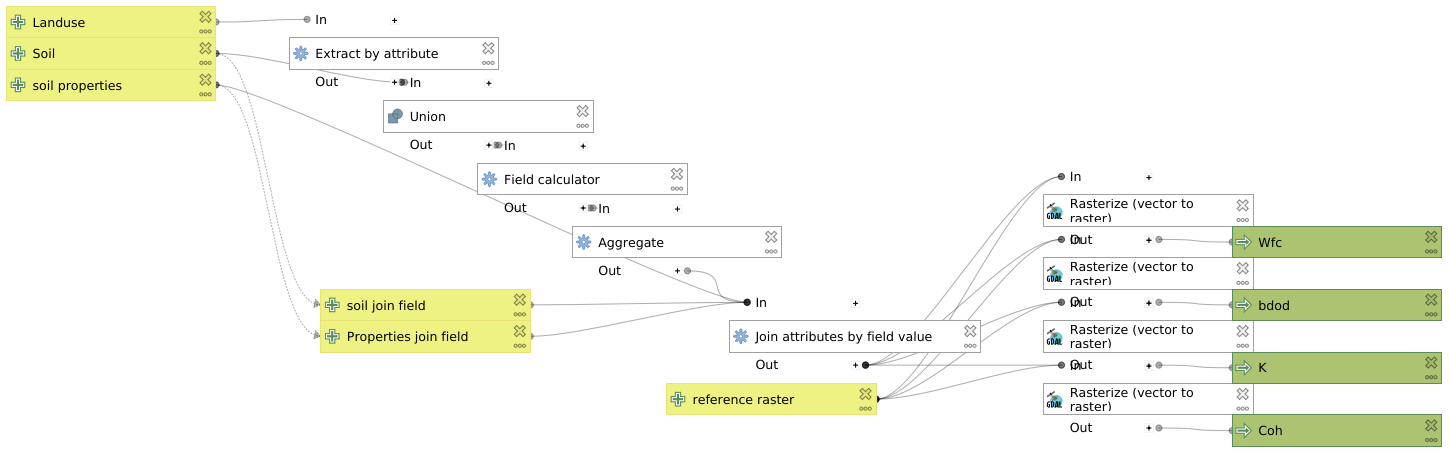
   Your final model should look like this:

   

2. Finally, rasterize the results. For reference, see Rasterizing the results:

   Field to use for a burn-in value [optional]	Rasterized	Description
   Wfc	Wfc	Soil wetness at field capacity \(%\)
   bulk_density	bdod	Soil bulk density \(\frac{Mg}{m^3}\)
   K	K	Soil detachability \(\frac{g}{J}\)
   Coh	Coh	Soil cohesion \(kPa\)

   Final model

   

Warning

Check that all values of the rasters you have created are the same as in the Hadocha_data.xlsx file before moving on! Also, it is very important that the rasters align exactly with Hadocha_dem, otherwise, you will get errors in the gdalrastercalculator. This should be good if you followed this manual.