4.3. Processing the data in the MMF model

Now it is time to start processing our data. We will describe fully how to implement the first set of equations. We will be making quite some small models that can later all be combined into one big model. This will help in debugging.

4.3.1. Estimating effective rainfall (\(P_e\))

The rainfall kinetic energy (\(KE [\frac{J}{m^2}]\)) is a function of effective rainfall (\(P_e\) ), i.e. the fraction of mean annual rainfall (\(P\)) that is not intercepted by vegetation (\(A\)). Thus:

(4.2)\[P_e = P(1-A)\]

1. Create a new model

2. Give it two Raster Layer inputs: P and A

3. Drag in a gdalrastercalculator or a qgisrastercalculator.

   GDAL:

   Fill in the following:

   • Input layer A: A

   • Number of raster band for A: 1

   • Input layer B: P

   • Number of raster band for B: 1

   • Expression: B*(1-A)

   • Calculated: : Pe

   Native:

   Fill in like so:

   • Expression: "P@1"*(1-"A@1")

   • Reference Layer(s): A or P

   • Output: Pe

   Notice the difference in Expression between the two. Because we are directly using inputs, the expression in is still relatively compact. However, if you start stacking algorithms on top of each other, they may quickly become quite long

4. Optionally, set a default location for the output raster

5. Name the model 01_effective_rainfall and save it under a name

4.3.2. Leaf Drainage and Direct Throughfall

1. Create a new model named 02_leaf_drainage

2. Drag in the necessary raster layer inputs for the following equations:

   \[\begin{split}LD = P_e \cdot CC\\ DT = P_e - LD\end{split}\]

   Solution

   

4.3.3. Kinetic energy

1. Create a new model named 03_kinetic_energy

2. Drag in the inputs for the followinw equations:

   \[\begin{split}KE_{DT} = DT\cdot(11.9+8.7\log(P_i))\\ KE_{LD} = LD\cdot(18.80\cdot\sqrt{PH}-5.88)\\ KE = KE_{DT}+KE_{LD}\end{split}\]

   Where \(P_i=11\frac{mm}{h}\) is the rainfall intensity and \(PH\) is the plant height.

   Note

   In the gdalrastercalculator, you can use any Numpy functions, such as log10. or sqrt. Additionally, powers are written as: 2**3=8.

   Checkpoint

   Check that \(KE_{DT}\in[0,31254]\) and \(KE_{LD}\in[816,17840]\). (For a rainfall of 1744)

   Hint

   You can rename your algorithms, so that you can actually distinguish them! Otherwise, they will all be called “Calculated” from algorithm “Raster Calculator”:

   

4.3.4. Surface Runoff

Now, this will be a bit more complicated. For knowing the surface runoff on a pixel, we need to also know the surface runoff of all the pixels above it. This is a process called flow accumulation.

Note

There are some algorithms by GRASS and SAGA that can do this. However, since the algorithms for flow accumulation are different between versions, and algorithms do not allow for a weighted input, I made a plugin that we will be using that wraps the richdem utilities and makes them useable in QGIS.

The Soil moisture storage capacity \(S_c\) is calculated by

\[S_c = 1000 \cdot W_{fc}\cdot \rho_{bd}\cdot EHD\sqrt{\frac{ET_{c,adj}}{ET_c}}\]

Where \(W_{fc}\) is soil moisture, \(\rho_{bd}\) is Bulk density, \(EHD\) is effective hydrological depth and \(\frac{ET_{c,adj}}{ET_c}\) is the ratio of evapotranspiration.

The resulting estimate for surface runoff per pixel is then:

\[\begin{split}\delta SR = P\cdot \exp\left(-\frac{S_c}{P_0}\right)\\ P_0 = \frac{P}{n}\end{split}\]

where \(P_0\) is the mean rain per day: Annual rainfall \(P\) and number of rainy days \(n=160\).

1. Create a model implementing the above equations

2. Load the map for \(\delta SR\). It should look like this:

   

   Fig. 4.3 The values should be \(\delta SR\in[0,57]\)

   Next, we need to route the flow. That is: for each pixel we know the runoff, and we want to calculate how it flows over the catchment.

4.3.4.1. Flow accumulation using rdflowaccumulation

For this we will use the rdflowaccumulation algorithm. However, our DEM contains some flat areas and depressions from which the algorithm does not know where to direct the flow. For this, we will use the rddepressionfill algorithm.

1. In your model, drag in a rddepressionfill and set it to DEM (Create a new input). Default settings are good.

2. Drag in a rdflowaccumulation and fill it in like this:

   • input layer: "Output layer" from algorithm "rddepressionfill"

   • flow metric: Dinf

   • weights [optional]: "Calculated" from algorithm "SR"

   • Output layer: SR_acc

4.3.4.2. Flow accumulation using Catchment area

1. In your model, drag in a Fill sinks and set it to DEM (Create a new input). The minimum slope is good on default settings.

   Note

   SAGA is very specific when it comes to misaligned rasters. It can be that your rasters misalign by \(10^{-6}\) and it will give a The Following layers were not correctly generated error. Because of this, we will use gdalwarpreproject to align the dSR raster to the filled DEM, as explained in this blog <https://gis.stackexchange.com/a/422090/156742>, explained in this blog.

2. Drag in a gdalwarpreproject algorithm. Press Show advanced parameters and fill in the following:

   • Input layer: "Calculated" from algorithm "dSR"

   • Source CRS [optional]: "Calculated" from algorithm "dSR"

   • Target CRS [optional]: "Filled DEM" from algorithm "Fill sinks (wang & liu)"

   • Georeferenced extents of output file to be created [optional]: |processing|"Filled DEM" from algorithm "Fill sinks (wang & liu)"

3. Drag in a Catchment area (flow tracing) and fill it in like this:

   • Elevation: "Filled DEM" from algorithm "Fill sinks"

   • Flow Accumulation units: [0] number of cells

   • Weights: "Calculated from algorithm "SR"

   • Method: [3] Deterministic infinity This is the flow routing algorithm.

4. Run the model. If everything works correctly, you should get the following output:

   

   Fig. 4.4 Your values should be \(\in[0,800000]\)

   Now, we are not interested in how much flow accumulates in the river areas. We will say that for any cell with \(SR>1400\) this is a river area and set \(SR_{final}=0\) there.

5. Drag in a gdalrastercalculator. The expression you should fill in is: where(A<1400,A,0), using the numpy.where(). Make sure that Input layer A points to "Flow Accumulation" from algorithm "Catchment area":

   

   Tip

   If you find yourself filling in inputs all the time, you can create a new model, drag in the 04_surface_runoff algorithm, and selecting the inputs as paths to the rasters.

4.3.5. Estimate soil detachment by raindrops \(F [\frac{kg}{m^2}]\) and runoff \(H []\frac{kg}{m^2}]\)

Soil particle detachment by runoff \(H\) is given by:

\[H=10^{-3}\frac{2SR^{1.5}}{COH}\sin(S)(1-GC)\]

Where \(COH [kPa]\) is cohesion, \(SR [mm]\) (use SR_final ) volume of surface runoff, \(S [\text{rad}]\) is slope and \(GC [-]\) is fraction of ground cover.

1. Create a new model named 05_detachment

2. Drag in a DEM input and a terrain attribute algorithm.

3. Next, drag in a qgisrastercalculator and fill in the equation. ( does not properly mask nodata values here and gives an “overflow encountered error” here. This is safe to ignore)

Solution

If you have filled in A : SR, B : COH, C : "Slope" from algorithm "Slope", D : GC, then the final expression is:

0.0005*A**1.5/B*sin(deg2rad(C))*(1-D)

It could be that does not like raising to a power. Then, you could try the raster calculator.

The final value should be \(H\in[0,1.2]\)

Soil particle detachment by raindrops, \(F\) is given by:

\[F=10^{-3}K\cdot KE\]

where \(K [\frac{g}{J}]\) is the soil detachability index and \(KE [J]\) is kinetic energy determined in Kinetic energy.

1. Add this calculation to the model

4.3.6. Calculating transport capacity and final erosion

Since we will also be using the slope in this model, we will be making the rest of our calculations in the same model.

The transpor capacity is given by:

\[TC = 10^{-3}C_fSR^2\sin(S)\]

Again, I used a qgisrastercalculator to calculate \(SR^2\), and filled this in into the model.

Next, the final erosion is given by:

\[E = \min(F+H, TC)\]

Use the minimum() to calculate this in gdalrastercalculator.

Solution

The final model looked like this for me:

Fig. 4.5 The final model layour for detachment and erosion

And the final erosion map looked like this:

Fig. 4.6 Values are between \(0,14.9\)

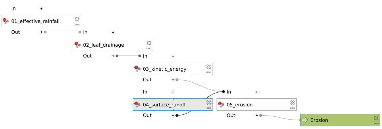
4.3.7. Putting everything into a single model

Now, you can create a new model and drag all the algorithms into it! Make sure to only set inputs as paths to files where they are acutally inputs from pre-processing. Otherwise use an Algorithm output from a previous algorithm. It should look like this: